
Raytracer
Raytracing is a computer graphics rendering technique for generating photorealistic images. The image is created by firing rays into the scene, which interact with objects in the scene. The rays interact with different surfaces and light sources which determine the final colour values of the pixels in the image.
For the final project of CS 488 (Introduction to Computer Graphics), I chose to extend the raytacer I had built in Assignment 4 with more advanced raytracing techniques. Unfortunately, the project was cancelled due to the COVID-19 shutdown. I continued to work on it on my own time and this page demonstrates its features.

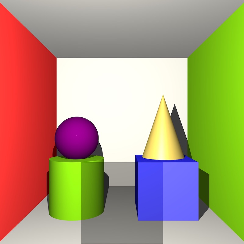
The raytracer supports plane, sphere, cube, cone, and cylinder primitives.
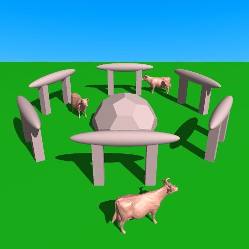
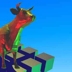
The raytracer supports triangle meshes via Wavefront OBJ files. In addition to 3D vertex coordinates, OBJ meshes can include texture coordinate indices and vertex normal indices.
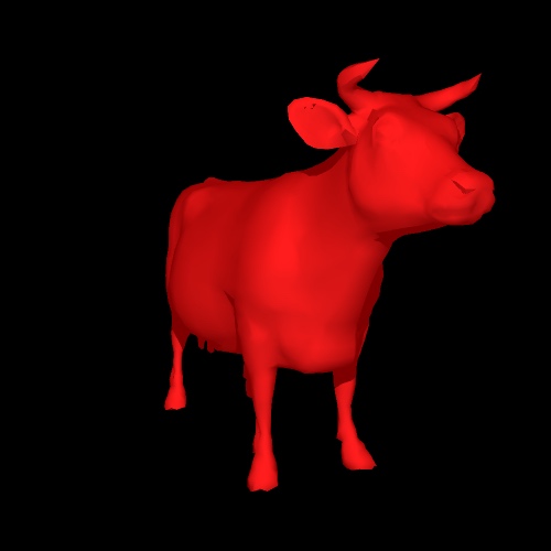
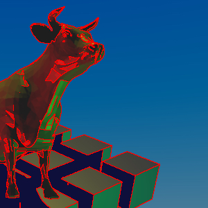
The following image features dodecahedron and cow meshes.
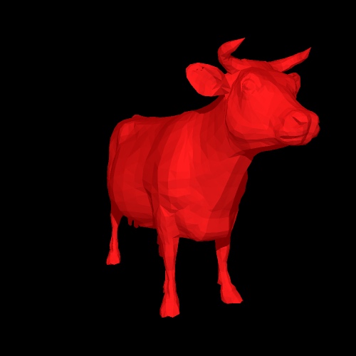
For meshes with included vertex normals, the raytracer interpolates the intersection normals using barycentric coordinates to give meshes a smooth look.
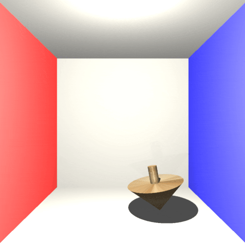
Flat shading on the left, Phong shading on the right.
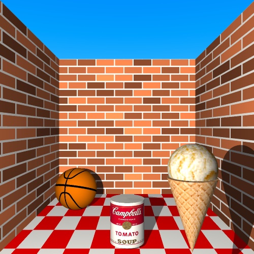
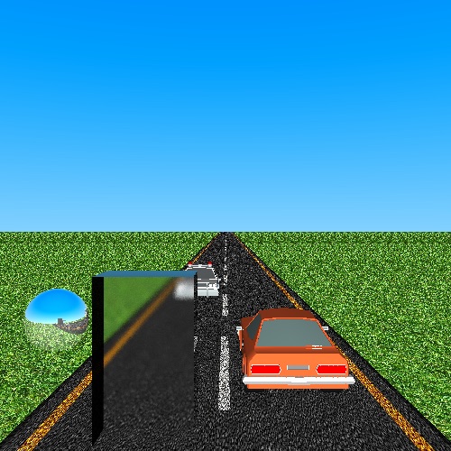
Texture mapping is implemented assigning UV coordinates when a ray intersects objects. Texture mapping works on most primitives as well as meshes with UV mappings. The normalized UV coordinates get mapped to a pixel on the original texture image using nearest neighbour interpolation. Texture mapping supports PNG images as well as primitive textures like checkered and striped patterns.
Primitive texture mapping on the left, mesh texture mapping on the right.
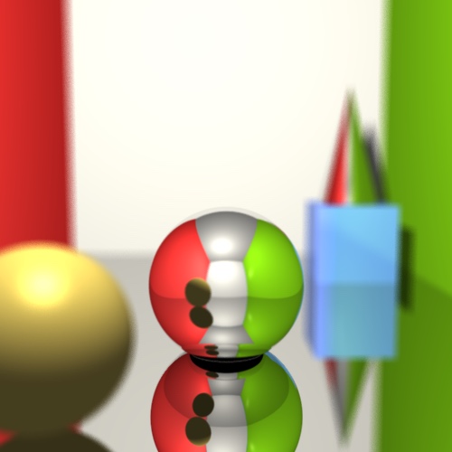
The raytracer supports regular and glossy reflection. When a ray hits a reflective object, a secondary ray is fired using the law of reflection. For glossy materials, several secondary rays are fired with some random perturbation and the average result is used. An upper threshold is used to limit the number of recursively-fired rays.
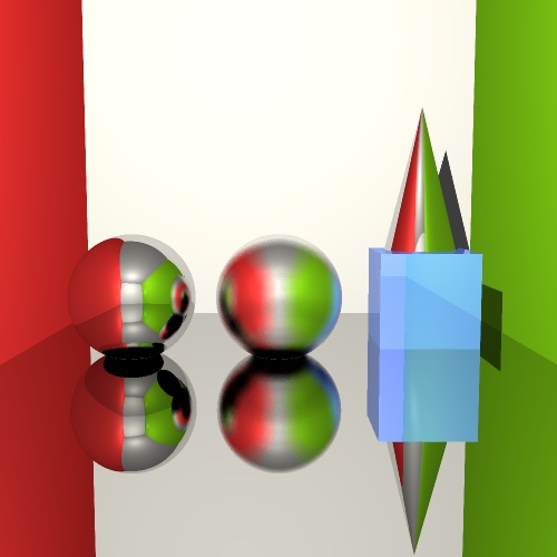
The raytracer also supports regular and glossy refraction. When a ray hits a transparent or translucent object, a secondary ray is fired into the material using Snell's law and the material's index of refraction. The Fresnel Effect can be observed on objects that exhibit both reflective and refractive properties. As with reflection, refraction in glossy materials is achieved by firing multiple secondary rays that are randomly perturbed.
Regular refraction on the left, glossy refraction on the right.
The raytracer supports depth of field by replacing the pinhole camera with a square camera lens. The depth of field effect is controlled by two parameters: focal length and aperture size. These parameters determine the convergence point where all primary rays intersect. Multiple secondary rays are generated by taking the origin to be a random point on the lens and the direction to be the convergence point. These rays are cast into the scene, where they are then averaged.
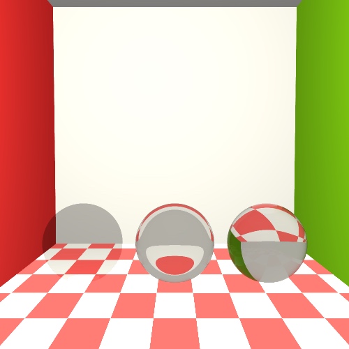
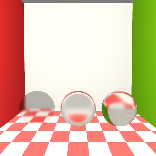
Adaptive supersampling is an antialiasing technique to selectively smooth out jaggies in the final image. It is achieved by initially sampling every pixel performed by dividing each pixel into four areas and sampling rays to the centres of those areas. If the resulting colour values differ from the colour of the centre point by more than some threshold, then that area is split into four additional quadrants and further sampling is performed.
No supersampling on the left, supersampling on the right, highlighted supersampled points in red on the bottom.

Animation is achieved by using Lua to render multiple frames and FFmpeg to stitch them together into a looping GIF.
Several optimization techniques are used to speed up rendering times:
- Multithreading
- Mesh bounding volumes Mesh rendering is accelerated by enclosing every mesh object in a tightly-bound box. Instead of testing for ray-intersection with every triangle in the scene, the raytracer tests against the bounding volume boxes. If the ray intersects with a bounding volume, then it will check for the nearest intersection of all the triangles within the box. Otherwise, all of the triangles belonging to the mesh will be skipped.
- 3D grid acceleration Mesh rendering is further optimized by dividing the bounding volume boxes into voxels. These voxels store pointers to the triangles of the mesh that are partially or fully inside them. Rather than testing for ray-intersection with every triangle inside the bounding volume, the raytracer only tests against the triangles in the voxels that the ray passes through. This is achieved using a 3D digital differential analyzer algorithm.
- Adaptive antialiasing As discussed earlier, a lot of unnecessary supersampling is skipped by selectively choosing which pixels to cast additional rays towards.
The raytracer uses multithreading to split up the work between all of the computer's CPU cores. The number of threads created is equal to the number of CPU cores. To achieve a fairer distribution of work among cores, pixels are assigned to threads in an alternating manner.
Some crude benchmarks were performed on a test scene consisting of several primitives as well as two meshes (9,392 triangles in total). The output image has a resolution of 500x500. Supersampling and depth of field effects were not used to render the final image. Glossy reflection and refraction used 30 perturbed rays.
Computer specs: MacBook Pro (Mid 2014), 2.2 GHz Quad-Core Intel Core i7-4770HQ
The following table compares the render times of the test scene using different combinations of optimization techniques.
| Multithreading | Bounding volumes | 3D grid acceleration | Time |
|---|---|---|---|
| 110m28s | |||
| ✓ | 20m4s | ||
| ✓ | 2m50s | ||
| ✓ | ✓ | 32s | |
| ✓ | ✓ | 14.5s | |
| ✓ | ✓ | ✓ | 4.1s |